PyCVF by Example

This is a preliminary help. It needs to be improved a lot. Please send us our comments.

Command line programs

Installing/listing/removing standard Datasets

PyCVF comes with a tool that help you to install standard database on your computer

pycvf-admin install-dataset WANG
pycvf-admin install-dataset CALTECH256
pycvf-admin install-dataset VOC2006
pycvf-admin listdb
pycvf-admin removedb WANG

Browsing datasets

Display default database:

pycvf

Display browsing one of the database you have installed:

pycvf -d 'official_dataset("WANG")'
pycvf -d 'image.caltech256()'

Note that the expression after “-d” is a python expression that is evaluated in a particular context (See Builders).

Displaying the content of a directory:

pycvf -d 'image.directory(select_existing_folder())'

Displaying the content from the web:

pycvf -d 'web.IPA("zoo","video")'
pycvf -d 'web.yahoo_image("tomato")'
pycvf -d 'web.youtube("conan")'

Note that the argument of “-d” is a Python expression, that is normally evaluated by using a lazy autoloader for modules. It means that Python will look at within a specialized context if the words you are using are already defined and it will also try to load objects from different paths if such a word is not found.

Some database come with some special object that help manipulating them:

pycvf -d "image.caltech256()" # whole caltech 256
pycvf -d "image.caltech256(5)" # 256 classes containing only 5 instances each
pycvf -d "image.caltech256(10,20)" # 20 classes containing only 10 instances each

Extract all ‘tomato’ image from yahoo image and divide each image into 9 pieces:

pycvf -d "exploded(web.yahoo_image('tomato'),pycvf.structures.spatial.Subdivide((3,3,1)))"

For complex databases that you use often you may create new database file to implement them:

from pycvf.databases.image import directories
from pycvf.databases import limit
from pycvf.datatypes import image

D="/databases/101ObjectCategories/PNGImages/"
datatype=lambda:image.Datatype
__call__=lambda:directories.__call__(D,dbop=lambda x:limit.__call__(x,30),rescale=(256,256,'T'))

Using models

** A model is a network of node which aim at transforming the reprensention of the information you are manipulating **

For instance we may want to apply some geometrical warp to our image

pycvf_features_view -d 'official_dataset("WANG")' -m 'image.map_coordinates("-x")' -i 1
pycvf_features_view -d 'official_dataset("WANG")' -m 'image.map_coordinates("x*2")' -i 1
pycvf_features_view -d 'official_dataset("WANG")' -m 'image.map_coordinates("x/2")' -i 1
pycvf_features_view -d 'official_dataset("WANG")' -m 'image.map_coordinates("x*1J")' -i 1
pycvf_features_view -d 'official_dataset("WANG")' -m 'image.map_coordinates("x**2")' -i 1
pycvf_features_view -d 'official_dataset("WANG")' -m 'image.map_coordinates("numpy.exp(x)")' -i 1
pycvf_features_view -d 'official_dataset("WANG")' -m 'image.map_coordinates("numpy.log(x)")' -i 1

The “-i” option is there to specify the interval of time in-between each entry of the database. Or if you want to compute and visualzie the HOG descriptors of the image in a folder you may do

pycvf_features_view -d 'image.directory(select_existing_folder())' -m 'image.descriptors.HOG()' -i 0.5

You may call any node defined in the nodes directory. Some of these nodes are poweful wrappers to other toolkits. You may use them to call any function in the specified toolkit. The free function allows you to apply any function that you may call from python. The string is assumed to be python expression where x is the object that you manipulate.

Nodes maybe combined together using the pipe operator “-“

pycvf_features_view -d 'image.directory(select_existing_folder())' -m 'free("x**2")-image.edges.laplace()-free("x**.5")'  -i 1

Computing features

You may save the result of this computation by using “pycvf_save” , or by using a node like “to_trackfile”

pycvf_save -d 'image.directory(select_existing_folder())' -m 'image.descriptors.HOG()' -o "trackHOG.tf" -p 8 #HOG
pycvf_save -d 'image.directory(select_existing_folder())' -m 'image.descriptors.LBP()' -o "trackLBP.tf" -p 8  #LBP
pycvf_save -d 'caltech256()' -m 'image.descriptors.CM()' -o "trackLBP.tf" -p 8 # color moments
pycvf_save -d 'caltech256()' -m 'image.descriptors.GIST()' -o "trackGIST.tf" -p 8 #GIST

The -p option allow you to use many processors at the same time.

The free model allow you to manipulate data in python directly:

pycvf_save -d 'image.directory(select_existing_folder())' -m 'free("scipy.stats.entropy(x.ravel()**2)")' -t "trackfile.tf"

Computing Indexes and Querying Them

First example ::

MODEL=’image.rescaled((64,64,”T”))-free(“x.ravel()”)’ locate .jpg|grep .jpg$|head –lines=100|pycvf_build_index -d ‘image.files()’ -m “$MODEL” -s xx

pycvf_build_index will build an index by adding for each element of the database a list of keys associated to a list a values. By default, the value is the address of the current element in the database. But other kind of values may imagined. pycvf_build_index assume that each value / key to be indexed will correspond to a row in the result returned byt the computational model. When on

Here the model for reprensenting the images is very simple since it is directly a vectorial reprensention of the bitmap image. We simply reduce the image to a size of 64 by 64. “T” means that image will be truncated if the aspect ratio does not fit, and then we flatten this 64 by 64 RGB image into a 12286 dimensions vector.

The database files used here expect that the user will provide a listing of the files to open. The listing of file to open may come by stdin as it is the case in this example or by storing the result in a file.

You may then query the nearest neighbor by running pycvf_nearestneighbors_qtapp

locate .jpg|grep .jpg$|tail --lines=100|pycvf_nearestneighbors_qtapp -d 'image.files()' -m "$MODEL" -s xx

You may also browse the nearest neighbor graph in 3d, using pycvf_nearestneighbors_panda (Note that 3d may not work under VirtualBox)

locate .jpg|grep .jpg$|tail --lines=100|pycvf_nearestneighbors_panda -d 'image.files()' -m "$MODEL" -s xx -n 50

You may also use

MODEL='image.rescaled((64,64,"T"))-free("x.ravel()")'
locate .jpg|grep .jpg$|head --lines=100|pycvf_build_index -d 'image.files()' -m "$MODEL" -s xx

Extracting Video Shots

Extracting regular shots

cd ~/pycvf/demos
./download_demosdatas.sh
echo $PWD/datas/kodak_instamatic.mpeg |\
pycvf -d 'randomized(video.shots_of( video.files(),LN("video.keyframes.fixed",10,return_images=False, return_positions=True)))'\
  -m "debug.display()"

Here the shots are randomized... You may try to change the number of keyframes used to delimit the boudaries of segment : try to use values like 100 or 1000.

Extracting regular shots based on discontinuity keyframes

echo $PWD/demos/datas/kodak_instamatic.mpeg | pycvf -d 'randomized(video.shots_of( video.files(),LN("video.keyframes.matching_model",model=LN("free","numpy.mean(x[0][2])")-LN("difft")-LN("free","abs(x)"),threshold=30.2,hystersi s=-2,return_images=False, return_positions=True)))'  -m "debug.display()"

This time we take in account the way the global luminosity evolves. Every discontinuity in the luminosity greater than a specified amount will generate a keyframe, and hence will be the boundary of a shot.

Extracting stable keyframes :

One way to define stable keyframes is to describe them as the middle frame contain in an interval delimited by two discontinuous keyframes, hence

echo $PWD/demos/datas/kodak_instamatic.mpeg | pycvf -d 'video.shots_of( video.files(),LN("video.keyframes.matching_model",model=LN("free","numpy.mean(x[0][2])")-LN("difft")-LN("free","abs(x)"),threshold=30.2,hystersis=-2,return_images=False, return_positions=True))'  -m "video.keyframes.fixed(1)-debug.display()"

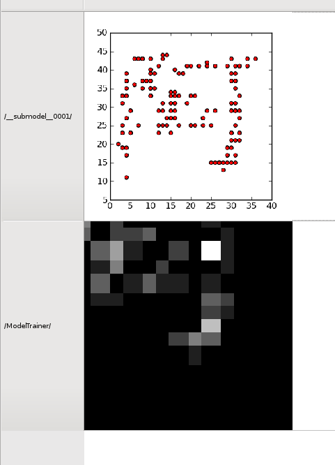
Density Estimators

This refers to the file : ~/pycvf/demos/shell_scripts/kanji_points.sh

To evaluate the perforamnce of different statistical model on learning manyfolds we observe the capacity that different statistical model have to learn a the shape some ideograms.

First of all here is the defintion of the database:

DB="vectorset.points_sampled_according_to_image(image.kanji(invert=True),48**1.3)"
pycvf -d "limit($DB,10)"

Then we use, different density estimator : and return the associated estimated density map

pycvf_features_view -d "limit($DB,15)" -m "naive()-naive()+vectorset.train_and_2dtestmap(ML('DE.histogram',(20,20),(0,0),(48,48)))"
pycvf_features_view -d "limit($DB,15)" -m "naive()-naive()+vectorset.train_and_2dtestmap(ML('DE.pyem_gmm',2,10))"
pycvf_features_view -d "limit($DB,15)" -m "naive()-naive()+vectorset.train_and_2dtestmap(ML('DE.parzen',2,10),48,48)"

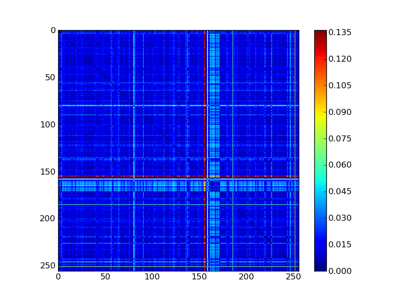
Computing Distance Matrices

The program pycvf_distance_matrix helps you to compute the distance matrices:

pycvf_distance_matrix -d "caltech101(3,numclasses=16)" --metric "lambda x,y:(((x-y)**2).sum()**.5)" -o dmmse.png
pycvf_distance_matrix -d "caltech101(3,numclasses=16)" --metric "lambda x,y:numpy.log10(1+(((x-y)**2).sum()**.5))" -o dmsnrlike.png

You may specify any python expression for performing the distance computation.

Using structures

Here are some simple examples

pycvf-admin install-dataset ZUBUD
pycvf_features_view  -d 'official_dataset("SZuBuD202")' -m 'exploded_transform(image.map_coordinates("numpy.log(x)"),LS("spatial").Subdivide((2,2,1)))' -i 1
pycvf_features_view  -d 'official_dataset("SZuBuD202")' -m 'exploded_transform(image.map_coordinates("x*1J"),LS("spatial").Subdivide((10,10,1)))' -i 1

Now we are going to create an index of these subimages based on HOG feature:

pycvf  -d 'exploded(official_dataset("SZuBuD50"),LS("spatial").Subdivide((8,8,1)),quick_len=True)' -A 1
pycvf_build_index -d 'exploded(official_dataset("SZuBuD50"),LS("spatial").Subdivide((8,8,1)),quick_len=True)' -m 'image.descriptors.HOG()' -s zubdubpartidx

Then we are going to transform each image in the “LFW” database by replacing each block by each nearest neighbor according to the descriptor HOG

pycvf-admin install-dataset LFW
pycvf_features_view -d 'exploded(official_dataset("LFW"),LS("spatial").Subdivide((8,8,1)),quick_len=True)' -m 'image.descriptors.HOG()-vectors.index_query_object(IDX("LoadIndex","/home/tranx/pycvf-datas/indexes/zubdubpartidx/"))'
pycvf_features_view -d "transformed(db=official_dataset('LFW'),model=LN('image.rescaled',(256,256,'T')))" -m "naive()-exploded_transform(image.descriptors.HOG()-vectors.index_query_object(LF('pycvf.indexes.load_index',LF('pycvf.indexes.sashindex'), '/home/tranx/pycvf-datas/indexes/zubdubpartidx/'), db=exploded(official_dataset('SZuBuD50'),LS('spatial').Subdivide((8,8,1)),quick_len=True))-free('pycvf.lib.graphics.rescale.Rescaler2d(thesrc[\"src\"].shape[:-1]+(\"T\",)).process(x[0][0])'), LS('spatial').Subdivide((8,8,1)))" -i 5 --all 1

This line may seem a little bit long and complicate, and it would be smart to create a simpler macro for this line, but it is interesting to see the elements that are present in this line, and to see how the generic components that have been use to resynthetize an object from database based on our database may actually be used in any system.

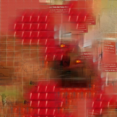
Same thing with color moments

pycvf_build_index -d 'exploded(official_dataset("SZuBuD50"),LS("spatial").Subdivide((8,8,1)),quick_len=True)' -m 'free("x/256.")-image.descriptors.CM()-free("x.ravel()")' -s zubdubpartidxCM
pycvf_features_view -d "transformed(db=official_dataset('LFW'),model=LN('image.rescaled',(256,256,'T')))" -m "naive()-free('x/256.')-exploded_transform(image.descriptors.CM()-free('x.ravel()')-vectors.index_query_object(LF('pycvf.indexes.load_index',LF('pycvf.indexes.sashindex'), '/home/tranx/pycvf-datas/indexes/zubdubpartidxCM/'), db=exploded(official_dataset('SZuBuD50'),LS('spatial').Subdivide((8,8,1)),quick_len=True))-free('pycvf.lib.graphics.rescale.Rescaler2d(thesrc[\"src\"].shape[:-1]+(\"T\",)).process(x[0][0])'), LS('spatial').Subdivide((8,8,1)))" -i 5 --all 1

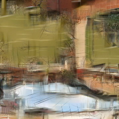
The results shall provide images like this:

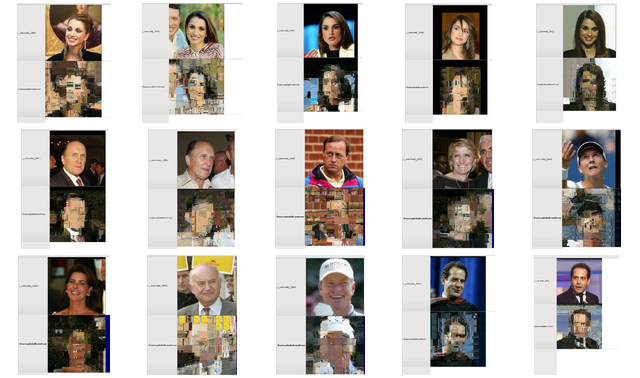
This line may seem a little bit long and complicate, and it would be smart to create a simpler macro for this line, but it is interesting to see the elements that are present in this line, and to see how the generic components that have been use to resynthetize an object from database based on our database may actually be used in many system, and maybe parametrized nicely.

At first shell scripts can help in getting more readable code

##
## normal retexturing
##

STRUCTURE="LS('spatial').Subdivide((8,8,1))"
FEATURE="free('x/256.')-image.descriptors.CM()-free('x.ravel()')"
IDXSTRUCT="LF('pycvf.indexes.load_index',LF('pycvf.indexes.sashindex'), '/home/tranx/pycvf-datas/indexes/zubdubpartidxCM/')"
ORIGDB="exploded(official_dataset('SZuBuD50'),$STRUCTURE,quick_len=True)"
SELECTRESULT="free('x[0][0]')"
ADAPTBACK="free('pycvf.lib.graphics.rescale.Rescaler2d(thesrc[\"src\"].shape[:-1]+(\"T\",)).process(x)')"

pycvf_features_view -d "transformed(db=official_dataset('LFW'),model=LN('image.rescaled',(256,256,'T')))" \
                    -m "exploded_transform($FEATURE-vectors.index_query_object($IDXSTRUCT, db=$ORIGDB,k=1)-$SELECTRESULT-$ADAPTBACK, $STRUCTURE)" \
                    -i 5 --all 1

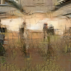
By modifying Structure, withouth changing the algorithm you can improve the algorithm

##
## smooth retexturing
##


STRUCTURE="LS('spatial').RegularOverlappingPatches((32,32),(16,16))"
FEATURE="free('x/256.')-image.descriptors.CM()-free('x.ravel()')"
IDXSTRUCT="LF('pycvf.indexes.load_index',LF('pycvf.indexes.sashindex'), '/home/tranx/pycvf-datas/indexes/zubdubpartidxCM1/')"
ORIGDB="exploded(official_dataset('SZuBuD50'),$STRUCTURE,quick_len=True)"
SELECTRESULT="free('x[0][0]')"
ADAPTBACK="free('pycvf.lib.graphics.rescale.Rescaler2d(thesrc[\"src\"].shape[:-1]+(\"T\",)).process(x)')"


pycvf_save -d "$ORIGDB"   -m "$FEATURE" -p 8 -t zubdubpartidxCM1 --pmode 1
pycvf_build_index -d "from_trackfile('zubdubpartidxCM1')" -s zubdubpartidxCM1
#pycvf_build_index  -d "$ORIGDB"   -m "$FEATURE" -s zubdubpartidxCM1

pycvf_features_view -d "transformed(db=official_dataset('LFW'),model=LN('image.rescaled',(256,256,'T')))" \
                    -m "exploded_transform($FEATURE-vectors.index_query_object($IDXSTRUCT, db=$ORIGDB,k=2)-$SELECTRESULT-$ADAPTBACK, $STRUCTURE)" \
                    -i 5 --all 1

To be continued...

Training Classifier and Computing Confusion Matrices

When working with complex database expressions, it may be useful to define variable for the database:

DB="transformed(db=as_once(lambda:limit(transformed(aggregated_objects(transformed( db=from_trackfile('CM',datatype=LF('pycvf.datatypes.basics').NumericArray.Datatype),model=LN('free','numpy.array([numpy.array(x,dtype=object).ravel()],dtype=object)'))),model=LN('free','numpy.vstack([numpy.hstack(reduce(lambda b,n:b+[n[0][1],n[0][2]],x[j][0][1],[])) for j in range(5)]).reshape(1,-1)')),256),label_op=lambda x:numpy.array([x],dtype=object)),model=LN('vectorset.whiten'))"

The simplest way to get a confusion matrix is to call vectorset.train_classification_and_confusion_matrix

pycvf -d "$DB" -m "LN('vectorset.train_classification_and_confusion_matrix',ML('CLS.weka_bridge','weka.classifiers.functions.LibSVM'),label='default_',label_op=lambda x:numpy.array(x[:,0],dtype=object))"
pycvf -d "$DB" -m "LN('vectorset.train_classification_and_confusion_matrix',ML('CLS.weka_bridge','weka.classifiers.meta.AdaBoostM1'),label='default_',label_op=lambda x:numpy.array(x[:,0],dtype=object))"
pycvf -d "$DB" -m "LN('vectorset.train_classification_and_confusion_matrix',ML('CLS.weka_bridge','weka.classifiers.trees.J48'),label='default_',label_op=lambda x:numpy.array(x[:,0],dtype=object))"
pycvf -d "$DB" -m "LN('vectorset.train_classification_and_confusion_matrix',ML('CLS.weka_bridge','weka.classifiers.trees.RandomForest'),label='default_',label_op=lambda x:numpy.array(x[:,0],dtype=object))"

More

With 200 nodes and 100 database component we can do much more... Have a look at the demo folder in your PyCVF directory.